Melanoma

Having learnt the basics of Deep Learning, I was looking for a project to consolidate and extend my knowledge. This Manning “Live Project”,"Semi-supervised deep learning with GANS for Melanoma Detection"caught my eye. GANS or generalized adversarial networks are a relatively new discovery dating from 2014 and have caught the public eye recently with their ability to generate deep fakes. However, they have other uses... One of the drawbacks of Deep Learning is the need for a large labelled dataset. The promise of GANS is they allowed Deep Learning with far smaller training sets. I was keen to learn more!
The Live Project provides a graduated series of tasks and references to useful readings. Apart from that I am on my own!
MNIST classifier
The first task in the project is to write a MNIST classifier with PyTorch that achieves at least 95% accuracy on the test set. The MNIST dataset is a large database of labelled handwritten digits often used to test machine learning algorithms. It is described as the “Hello, world!” of Deep Learning, but I think this is a poor analogy. Although, a MNIST classifier is often the first task that an individual new to Machine Learning tries, the complexity of the task is magnitudes higher than a “Hello, world!” program.
The mechanics of the maths is relatively simple. The main mathematical techniques used are multivariate calculus, linear algebra and gradient descent optimisation – techniques that are typically covered at say the 2nd year undergraduate level. But ML maths asks deeper questions. Why is stochastic gradient descent (‘SGD’) more effective than gradient descent for this problem? Why do some simple neural networks generalise beautifully and work on data that is not in the training set? The answers to some questions are deep. For other questions we do not have satisfactory answers. As a result, the general approach to ML is a mixture of intuition and experiment.
On the surface PyTorch is simple as well, but behind the surface is some amazing engineering. At its heart, PyTorch is a Python library that provides multi-dimensional vectors, called tensors. But the tensors carry some metadata with them. When mathematical operations are performed on the tensors, behind the scenes a DAG is created. And each tensor has a backward function on it. If the backward function is called, then the DAG is walked in reverse and the derivatives of the tensor w.r.t. the parameters are calculated using the multivariate chain rule. The derivatives are used by the SGD optimiser to adjust the input parameters. Further, as well as running on a standard CPU, PyTorch is also optimised to run on a GPU.
My goal was to aim for a relatively simple classifier that was still able to achieve a high degree of accuracy. I used a convolutional neural network (CNN) with two convolutional layers, two pooling layers, one fully connected linear layer and one dropout layer. I borrowed this topology from a MITx course. It proved very effective achieving 99.1% accuracy on the test set. I experimented with tweaking some of the parameters and this did not improve the accuracy, so I expect quite a lot of work had already gone into this design.

Although the performance of this classifier is very good, it is not perfect. It is interesting to look at some of the digits it failed to classify. Some are almost incomprehensible and a human would struggle with them. Others though are easily classified by people. Sometimes a very heavy pen has been used, sometimes the digit has been written on an angle, sometimes an extra loop has been added. It is of concern, that very small things can prevent digits being classified accurately.

Baseline Melanoma classifier
The next task was to write an initial baseline model to detect melanoma. The catch is that the balanced training set is only 200 images. The balanced test set was 600 images. And a further 7018 unlabelled images were provided. The images are low resolution three channel 32 x 32 pixel images.

The model has around 60K parameters so as expected was prone to rapidly start overfitting. Nonetheless I achieved an accuracy rate of 68%, which given the paucity of data, I was pretty pleased about. But could this result have come about by chance? The given the size of the test set, I thought it was unlikely. But best still to check:

Augmented Melanoma classifier
To further improve the performance, I then augmented the dataset based using 4 random rotations and 2 flips. Augmenting the dataset helps to address the fact that the dataset may be unrepresentative. Following, augmentation the accuracy increased 3% to 71%.
Using Transfer Learning for the Melanoma classifier
It turns out that within the field of image recognition, using a model with another dataset can be very effective. Although at first this seems couterintuitive, in turns out that a lot of convolutions - such as edge detectors - are useful universally.
I started with the well known resnet18 model, which is 8 layers deep. The model had been pre-trained on the ImageNet database consisting of over 1million images. However, out of the box the models assigns images to one of a thousand categories such as "golden retriever". However, for the Melanoma project, I needed a binary classifier. I add a fully connected layer consisting of a single neuron and a sigmoid activation function. I then trained the additional weights I had added, but froze the pretrained weights. This proved effective, increasing the accuracy rate of the augmented Melanoma classifier from 71% to 78%.
A Jupyter notebook containing all three models is available here.
The instructor also achieved around 71% on her augmented Melanoma classifier. However, she was suprised that it was that good with only 140 samples (60 reserved for the validation set) and feels that the melanoma negative images are often in a warmer shade. If this is correct, then it makes the whole project problematic. If the test accuracy increases with a GAN assisted classifier, could it not just be exploiting the existing bias in the data better?
MNIST Image generators
MNIST variational autoencoder
Before building a GAN, we were set a task to generate images based on the MNIST dataset using a simpler generator - a variational autoencoder.
An autocoder is basically a neural network that is trained against its own input. But the thing that prevents it becoming a null operation, is that it contains a bottleneck called the latent space. The latent space is a fully connected row of neurons that have a lower dimension than the input. The lower the dimension, the more the autoencoder will compress the image. The part of the neural network between the input and the latent space is the encoder and the part between the latent space and the output is the decoder. As well as compress images, autoencoders can be trained for other image enhancement tasks. For example, if Gaussian noise is added to the inputs they can be trained to denoise images. Likewise they can be trained to recolour images or sharpen images.
The variational autoencoder makes the latent space a stocastic layer. Rather than be a set of neurons, the latent space samples numbers from the multivariate Gaussian distribution whose mean and variance are controlled by the encoder. There is a clever mathematical trick to ensure that backpropogation works through the stocastic layer. (Details are in Kingma and Welling's well known paper, "Auto-Encoding Variational Bayes"). The other difficulty is that training the neural network will soon bring the variance down to zero removing the stocastic element. To prevent this, the loss function needs to be adjusted. The Kullback-Leibler divergence between the distribution of the latent space and the standard Gaussian distribution is added into the loss function. This ensures that the neural network is optimised to recreate the input whilst keeping the latent space stocastic. Once trained, if vectors of random numbers are given to the decoder, it will produce output that tries to mimic the output on which it was trained.
Coding up the MNIST variational autoencoder was straightforward and I soon had it generating example digits.
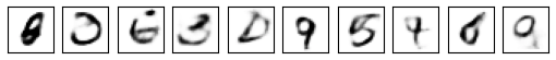
The results are slightly disappointing. Although some images are clearly recognisable as digits, other are mere digit like shapes.
MNIST GAN
The next task was to build a GAN to generate MNIST digits. GANS were introduced in June 2014 by Ian Goodfellow etal in the paper "Generative Adversial Networks".
A GAN consists of a pair of neural networks. One, the generator, aims to create something - in this case MNIST digits. The other, the discriminator, aims to tell genuine output from fake output. Both neural networks are trained iteratively in lock step. The discriminator is fed a mini-batch consisting of real digits and fake digits generated by the generator and its weights are optimised. Then the generator is fed a mini-batch of random numbers and its weights are optimised depending on whether the generator can correctly classify its output. This process is repeated iteratively. The result is a min-max two-player game between the two neural networks, which is optimised when Nash equilibrium is reached.
I first built a simple linear generators and discriminator. Results were similar to the variational autoencoder.

MNIST DCGAN
I then constructed a DCGAN or deep convolutional GAN. As their name implies, they have convolutional layers in the discriminator. They also have convolutional transpose layers in the generator. Researchers stuggled to train DCGANs until Radford etal's 2015 paper "Unsupervised Representation Leaerning with deep Convolutional Generative Adversarial Networks", which recommended batch normalization after each layer and also leaky ReLU instead of standard ReLU.
And I found training the DCGAN particularly tricky. In my case, it turned out I had an unexpected interaction between PyTorch's eval mode and the batch normalisation layer. It also took roughly 2 hours to train on my CPU. However, there is a noted step up in the quality of digits that it generates. Most of the digits are now indistinguishable from the training data. The notebook is here.

Melanoma classifier
The approach to Melanoma classifier is to build a semi-supervised GAN ('SGAN') where the discriminator makes a three way determination: fake mole, negative for melanoma and positive for melanoma. Labelled data is fed into the discriminator and marked positive or negative as appropriate. Fake images from the generator are marked as fake and unlabelled images are marked as real.
Initially the discriminator had two output layers consisting of single neuron with sigmoid activation layers. One neuron represented if the mole was malignant or benign. The other neuron whether the image was a real or a fake image. However, I found that this version of the SGAN was not any more accurate than the CNN. Then following a suggestion in Olga Petrova's article, "Semi-Supervised Learning with GANs: a Tale of Cats and Dogs", I switched to the approach advocated by Saliman et al in "Improved Techniques for Training GANs".
The authors start by suggesting an output layer consisting of three neurons with a softmax activation layer: one neuron represents a malignant melanoma, one neuron a benign melanoma and the third neuron a fake image of a mole. They then point out that the layer is over parameterised and the third neuron can be dropped and instead replaced with a value hard wired to zero.
This was effective and switching from a CNN to a SGAN and making use of the additional unlabelled data resulted in an increase in test accuracy from 71% to 76%. Even allowing for the effects of hyperparameters and the stochastic nature of the models, I believe this is definitely an improvement in performance. I had expected a larger improvement in accuracy, but believe the improvement was relatively modest due to the unexpectedly high performance of the supervised CNN.
One final point. The test accuracy is a very simple measure of the performance of the model. A better metric would be AUC-ROC, which is measures how well the model trades off specificy and sensitivity.
My Jupyter notebook for the model is here.
Summary
I have really enjoyed this live project and it has helped my growth as a Machine Learning Engineer. The MOOCs I have taken previously have given me the theoretical background: for example using the multi-variate chain rule and coding a simple neural network from scratch in Python. But they were less focussed on practical applications of Machine Learning.
Conversely, in this project I have learnt how to use GANs to create simulated images, but I have also learnt so much more. I hadn't come across autoencoders, for example, which are an unsupervised technique that allow building a range of image utilities such as: lossy compressors, denoisers, sharpners and colourisation. But beyond that I have increased my understanding of deep learning. I have two techniques at my figure tips for use when there is insufficient data for standard deep learning (likely to be most real world scenarios): transfer learning and SGAN, both of which increased the accuracy of my classifier. In terms of executing the model, I have moved past running on my local CPU and have deployed models remotely on the CoLab GPUs.
And finally I have moved beyond the "out of the box" functionality in PyTorch. I have read journal articles, and in the case of the SGAN classifier, implemented the loss function myself.
Picture of the microscope courtesy of SFO Museum, San Francisco. Used under the Creative Commons CC BY-SA 2.0 licence.